Common architecture mistakes
Consider a team that builds a managed vector database and an embedding pipeline so employees can search a 40-page staff handbook. Another team runs LIKE '%term%' over two million documents and wonders why nobody uses the search box. Both skipped the same step: measuring the corpus and the workload before choosing an architecture.
Corpus size tells you which systems are viable. Query volume, filters, tenancy, freshness, and cost determine when you must change systems.
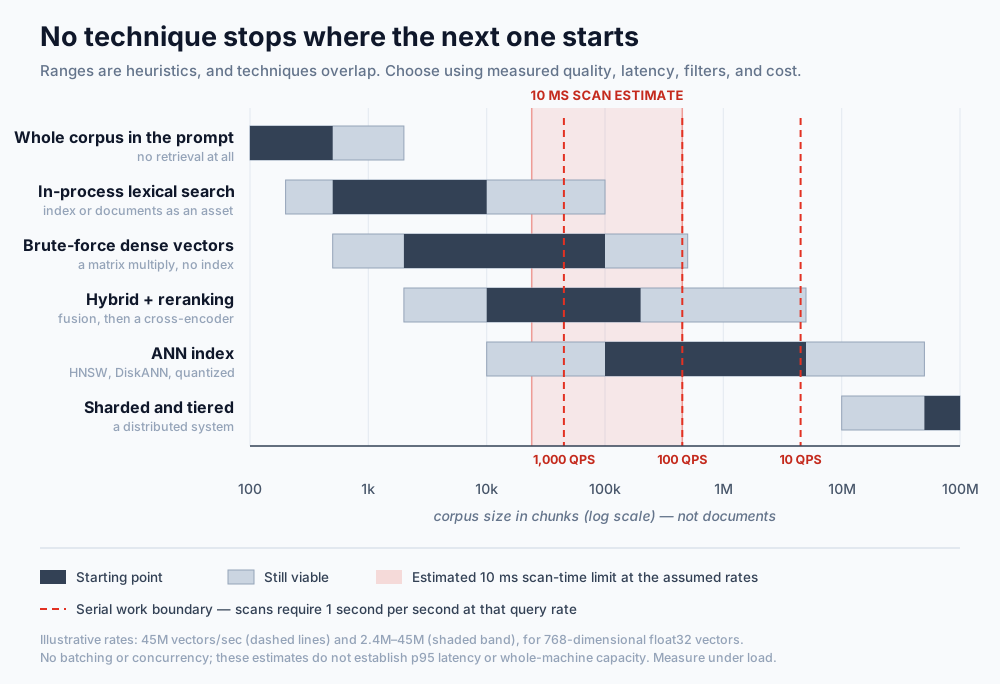 Search techniques plotted against chunk count on a logarithmic scale, with overlapping heuristic ranges. A shaded band shows illustrative 10 ms scan-time limits at assumed rates of 2.4M and 45M vectors per second. Dashed lines show where serial scan work reaches one second per second at 10, 100, and 1,000 QPS using the 45M rate. These are a model for article-concept illustration.
Count chunks instead of documents
Retrieval thresholds are usually expressed in chunks, while teams count documents. For the estimates below, one chunk means roughly 400 words of English prose. Use your actual chunk count if you already have one.
The multiplier varies far more than a single average suggests:
| Document type | Typical length | Chunks each (~512 tokens) |
|---|---|---|
| Support ticket, chat message, product record | Under 300 words | 1 |
| Knowledge-base article, FAQ entry | 500–800 words | 2–3 |
| Blog post, internal wiki page | 1,500–3,000 words | 4–8 |
| Long-form report, technical article | 4,000–6,000 words | 10–16 |
| Contract, policy manual, PDF handbook | 15,000+ words | 40–100+ |
A "10,000 document" corpus is anywhere from 10,000 to 500,000 vectors depending entirely on what those documents are. Overlap inflates the count further: at 512 tokens with 64 overlap the effective stride is roughly 448 tokens, adding about 15%. Compute your own number — total words ÷ 380 × 1.15 ≈ chunks — rather than relying on the table.
Tenant, workspace, and permission constraints can reduce the effective corpus when the execution plan selects matching candidates before scoring them. Filtering after ANN retrieval may provide much less reduction and can hurt recall.
Retrievers and reranking
Retrieval is often presented as a choice between keywords and embeddings. In practice, learned sparse retrieval is a third option, and reranking can improve all three.
| Technique | How it matches | Where it wins | Where it fails |
|---|---|---|---|
| Lexical (BM25) | Term overlap, weighted by term rarity and document length | Exact identifiers, names, error codes, SKUs, acronyms, with suitable tokenisation | Vocabulary mismatch when the query and document use different words |
| Dense (embeddings) | Cosine similarity, dot product, or another model-appropriate metric between independently encoded vectors | Paraphrase and conceptual similarity | Can miss exact identifiers; compare with lexical retrieval on your query set |
| Learned sparse (SPLADE, ELSER, OpenSearch neural sparse) | Learns term weights and expansion for documents, and often queries, scored through an inverted index | Semantic matching using inverted-index infrastructure | Quality and query-time inference requirements depend on the model |
| Reranking (cross-encoder) — orthogonal | Reads query and candidate together rather than comparing precomputed vectors | Improving the order of retrieved candidates | Cost and latency depend on candidate count, text length, model, and hardware |
Learned sparse retrieval deserves more attention than it typically receives. It delivers semantic matching — handling paraphrase and vocabulary mismatch — using inverted-index infrastructure, which means no vector index to operate, no embedding-serving infrastructure at query time, and exact metadata filtering that does not degrade with selectivity. For many teams at tiers 2 and 3, it offers the best quality-per-unit-complexity available, and almost nobody evaluates it. A cross-encoder reranker is orthogonal to all three techniques: it reads query and candidate together and can judge relevance that no pair of independently computed vectors can express, which is why it frequently outperforms swapping embedding models.
The six tiers
Use the last column as the migration test; the boundaries are working heuristics.
| Tier | Documents | Chunks | Approach | Signal you have outgrown it |
|---|---|---|---|---|
| 0: Prompt | 1–50 | Under 500 | The entire corpus in context. No retrieval. | Answer quality, latency, token cost, or context capacity |
| 1: In-process | 50–1,000 | 500–10k | Lexical search or brute-force cosine in memory; index or documents can be shipped as a static asset | Ranking quality, memory or payload size, or sustained query volume |
| 2: Hybrid + reranking | 1k–20k | 10k–100k | BM25 + dense with fusion when useful; brute force may suffice; start reranking around 50 candidates | Sustained query volume, or filters you cannot express |
| 3: Indexed | 20k–200k | 100k–2M | An ANN index; pgvector with HNSW is usually enough | Filtered recall you cannot fix, or RAM cost |
| 4: Dedicated | 200k–5M | 2M–50M | Purpose-built engine, quantization, disk or object-storage tiering | Cost per stored vector becomes the deciding factor |
| 5: Distributed | 5M+ | 50M+ | Sharding, tiering, and cost engineering as a discipline | You are past the scope of this article |
Tier 0 — the whole corpus in the prompt (under ~500 chunks)
If the corpus fits comfortably in the context window, test putting it in the prompt. This removes the chunking and indexing pipeline, but fitting does not guarantee good answers: long-context research shows that models can miss information within their supported windows. Measure accuracy, latency, and token cost. At 512 tokens each, 500 chunks occupy about 256,000 tokens, leaving limited room in all but the largest context windows.
Estimate cache cost from your expected hit rate, expiry policy, and update frequency. Providers may charge separately for reads and writes; Claude does. Frequent prefix changes make a cache-hit-only estimate optimistic. Compare the full request cost with the engineering cost of retrieval.
Options:
| Option | Pick it when |
|---|---|
| Whole corpus in a cached prefix | The corpus is static and fits comfortably in the window, with room left for the conversation |
| Table of contents in the prompt, full section fetched by tool call | The corpus is a filesystem, repository, or wiki with real structure, and most queries touch one part of it |
| Summaries in the prompt, full documents fetched on demand | The corpus nearly fits, and losing detail at the index layer is acceptable because the model can always ask for the original |
The last two options use tools for retrieval without requiring a vector index. Move to tier 1 when whole-corpus prompting misses your quality or latency targets, stops fitting, or costs more than a retrieval pipeline.
Tier 1 — in-process (500–10,000 chunks)
vgtc.io uses this approach below the tier's nominal range. At this revision, its 18 articles produce 183 article search documents: one summary per article and one entry per H2 section. Other site pages contribute additional search documents. Deploy time generates a static JSON file containing the documents; the browser downloads that file and builds the MiniSearch index when search is opened. Queries run in the browser without a search server, vector store, or embedding call.
| Option | Pick it when |
|---|---|
In-process lexical search — MiniSearch, Orama, or FlexSearch in JavaScript; bm25s, rank_bm25, or Tantivy in Python and Rust | Hold the index in memory; browser applications can download a serialized index or documents to index locally |
Brute-force dense — a NumPy matrix multiply, FAISS IndexFlat, hnswlib BFIndex, or usearch.index.search(..., exact=True) | Queries are paraphrase-heavy enough that term overlap misses them, and you already have embeddings |
SQLite with FTS5 and sqlite-vec, or DuckDB with vector distance functions | You want a queryable file for embedded apps, desktop tools, CLI tools, or offline use |
These lexical libraries do not all use BM25. FlexSearch, for example, uses position and context scoring. DuckDB's separate VSS extension adds HNSW indexing and is documented as experimental; assess that status before relying on it for a persistent production index.
Add a reranker when precision in the top five degrades. Move down to tier 0 when whole-corpus prompting meets the quality and latency targets at lower cost.
Tier 2 — hybrid plus reranking (10,000–100,000 chunks)
At this size, combine lexical and dense retrieval when the query mix justifies both, then rerank a small candidate set. Brute-force dense search may still work.
| Option | Pick it when |
|---|---|
Postgres — pgvector for dense, ParadeDB pg_search for BM25 | You already run Postgres. Avoids a separate service, while adding extensions and indexes to maintain; also worth evaluating at tier 3 |
| Elasticsearch or OpenSearch | You already run Lucene, or you want BM25, dense kNN, learned sparse, and RRF fusion in one system |
SQLite with FTS5 and sqlite-vec | Single-node application, embedded or offline deployment, one writer |
| Typesense or Meilisearch | You want built-in hybrid search and typo tolerance without operating Lucene |
| A reranker layered over any of the above | Top-result precision needs improvement; this is a layer rather than a store |
Rerankers are available as hosted APIs from Cohere, Voyage, and Jina, or as self-hosted cross-encoders such as the permissively licensed BGE family. Evaluate them against your data.
A dedicated vector database is usually unnecessary here. At 100,000 vectors, exact search can still be fast enough; ranking quality is more likely to be the constraint.
Move to tier 3 when scans exceed the p95 latency budget, query volume makes O(N) work too expensive, or the current store cannot support required filters. Move down when deduplication or narrower scope reduces the effective corpus below 10,000 chunks.
Tier 3 — indexed (100,000–2M chunks)
If you already run Postgres, start with pgvector; this corpus size alone does not require a dedicated vector engine.
| Option | Pick it when |
|---|---|
pgvector with HNSW | You already run Postgres and the index fits your latency, recall, and memory targets |
pgvectorscale (StreamingDiskANN) | Same Postgres, but the graph no longer fits the RAM |
| Elasticsearch or OpenSearch kNN | Faceting, highlighting, synonyms, analyzers, or multilingual tokenisation are product requirements — any one of these can determine the architecture |
| Qdrant | Selective filters cause unacceptable ANN recall in your current store |
| Typesense or Meilisearch | Their built-in hybrid search and ranking controls meet your product requirements |
| LanceDB | The corpus lives on object storage, query volume is modest, and cost at rest matters most |
| Managed — Pinecone, Vertex AI Vector Search, Azure AI Search, Cloudflare Vectorize | You prefer serverless solutions |
Before changing systems, test int8 or binary quantization with a full-precision rerank over the top candidates. Quantization can keep a tier 4-sized corpus on tier 3 hardware, though you must measure the effect on recall.
Move to tier 4 when filtered recall remains poor, RAM per vector eats the budget, or index rebuilds exceed the maintenance window. Deduplication or physical per-tenant partitioning can move the workload back to tier 2.
Tier 4 — a dedicated engine (2M–50M chunks)
Without our own benchmark, we will not rank these engines. Compare their storage and compute models instead:
| Family | Representative systems | Main cost |
|---|---|---|
| Dedicated engines with configurable memory and disk use | Qdrant, Weaviate | Compare the chosen index, compression, and cache settings; tail latency depends on the working set and workload |
| Distributed engines | Milvus, Vespa | Scale and adaptive execution, paid for in operational headcount |
| Object-storage-native | turbopuffer, LanceDB | Lower storage cost at rest, paid for in cold-query latency |
| Search engines at scale | Elasticsearch, OpenSearch with quantization | Keeps hybrid, facets, and analyzers when search is the product |
| Managed serverless | Pinecone | Buy instead of run; sets both the price floor and the lock-in |
These families overlap. Qdrant offers memory and disk placement controls, and Weaviate documents a disk-based HFresh index alongside HNSW. Compare specific configurations at the same recall target rather than inferring latency from the product name.
Quantization, deduplication, or tenant partitioning may bring the workload back to tier 3. Move up when a single shard is no longer sufficient.
Tier 5 — distributed (50M+ chunks)
At this scale, write rate, tenant skew, filter selectivity, and the ratio of hot to cold data matter more than corpus size. They lead to different architectures, so a generic shortlist would be misleading.
Many tier 5 stores are much smaller per query after tenancy is applied. Storing 100 million vectors and searching all 100 million for each query are different workloads. Physical partitioning or selecting candidates through a metadata index can reduce search work; post-filtering ANN candidates may not.
Choosing the operating model
Dense retrieval does not require a dedicated vector database. OpenSearch, Postgres, MongoDB, and SQLite all search vectors; the operational model matters as much as retrieval quality and scale.
| System | Use it when | Main drawback |
|---|---|---|
In-process (bm25s, MiniSearch, NumPy) | Tiers 0–1; lexical search or exact dense scans fit in application memory | The application manages loading, updates, concurrency, and persistence |
SQLite + FTS5 + sqlite-vec | Tiers 1–2; an embedded or offline app needs BM25 and exact dense search in one file | Single writer; no ANN index or horizontal scale |
Postgres + pgvector (+ ParadeDB pg_search) | Tiers 1–3; you already run Postgres and want full-text and dense search without another service | Native FTS is not BM25; extensions and indexes add maintenance |
| MongoDB Search + Vector Search | Tiers 2–4; documents already live in MongoDB and you want full-text, filtered vector, and hybrid search in one platform | Search uses separate indexes and resources; vector memory and dedicated Search Node costs can outweigh the one-platform convenience |
| Elasticsearch / OpenSearch | Tiers 2–4; you need BM25, ANN, hybrid fusion, facets, analyzers, or highlighting | JVM cluster overhead may be excessive for small corpora |
| Typesense / Meilisearch | Tiers 1–3; you want built-in lexical, dense, and hybrid search without operating Lucene | Check that the ranking controls, filters, and integrations fit the workload |
| Vespa | Tiers 3–5; the product needs complex, multi-phase ranking | Steep learning curve |
| Dedicated vector engines (Qdrant, Weaviate, Milvus) | Tiers 3–5; vector retrieval and filtered ANN justify a purpose-built engine | Lexical search, facets, highlighting, analyzers, and synonyms vary by engine |
In-process indexes can be persisted: MiniSearch supports JSON serialization, and bm25s supports saving and loading indexes. PostgreSQL's native ranking functions use different scoring methods from BM25; that distinction alone does not establish which will rank your results better.
A search engine provides faceting, highlighting, synonyms, analyzers, multilingual tokenisation, and aggregations. If the product needs these features, use a search engine even if corpus size alone would allow a simpler system.
OpenSearch's serverless variants trade cluster operations for billing constraints, which differ by product; check current pricing before provisioning.
The two crossovers
Brute force has two limits: per-query latency and sustained throughput.
The latency crossover
The latency crossover is where measured query latency exceeds the target, such as p95 below 10 ms. A single-query brute-force scan is often limited by memory bandwidth. A 768-dimensional float32 vector occupies 3,072 bytes, so reading N vectors once requires about 3 KB × N, excluding scores and other overhead.
For an example, assume a scan rate of 45 million vectors per second:
| Corpus | Assumed scan rate | Estimated scan time |
|---|---|---|
| 10,000 | 45M vectors/sec | ~0.2 ms |
| 100,000 | 45M vectors/sec | ~2 ms |
| 1,000,000 | 45M vectors/sec | ~20 ms |
At that rate, reading 3,072 bytes per vector implies roughly 140 GB/s of vector-data traffic if each vector is read once from main memory. Under the same linear model, a 10 ms scan-time allowance covers ~450,000 vectors. With a slower assumed rate of 2.4 million vectors per second, it covers ~24,000. Those two assumptions define the shaded band in the diagram.
Dimensions, data type, implementation, thread count, batching, and cache behaviour all affect scan rate. Measure p95 directly at the target sizes and leave room for the rest of the query path.
Quantization changes both the bytes read and the arithmetic. int8 components occupy a quarter of the space of float32 components, before scales and metadata, but do not guarantee fourfold faster search. Measure latency and recall with the implementation you plan to deploy, including any full-precision candidate rescoring.
The throughput crossover
At fixed dimensionality, brute force performs O(N) distance work per query. Q queries per second over N vectors require Q × N query-vector comparisons per second. In a serial, unbatched model, divide that product by the scan rate to estimate the scan time demanded in each elapsed second. Using the illustrative rate of 45 million vectors per second:
| Query rate | Corpus | Query-vector comparisons/sec | Estimated scan seconds per elapsed second |
|---|---|---|---|
| 10 QPS | 100,000 | 1M | ~0.02 sec |
| 100 QPS | 100,000 | 10M | ~0.2 sec |
| 1,000 QPS | 100,000 | 100M | ~2 sec |
| 100 QPS | 1,000,000 | 100M | ~2 sec |
Values above one mean that this serial scan model cannot keep up; they do not size a production deployment. Batching can reuse corpus data, while concurrency changes resource utilisation. Faiss documents these effects.
In this model, a 10 ms scan and 100 QPS meet at the same corpus size because 100 × 0.01 = 1: scans occupy all serial execution time. That is saturation with no headroom, not a p95 service guarantee. Measure sustainable QPS under representative load.
An ANN index can justify its cost at high traffic before isolated queries exceed the latency budget. Choose it from corpus size × query rate, not corpus size alone.
When ranking becomes the bottleneck
In the low tens of thousands of chunks, finding relevant candidates may remain easy while ordering them becomes harder. Recall@50 can stay high as precision@5 falls: the correct result is present, but too many plausible candidates rank above it.
This calls for a cross-encoder reranker over the top candidates, not another index.
Start with around 50 candidates, then tune the count against recall, ranking quality, latency, and cost. Cohere's API documentation recommends staying within 1,000 documents, but the practical limit depends on text length, model, batching, and hardware. A reranker cannot recover a document that retrieval omitted.
Your query mix is important
Different query types need different tools:
- Exact-term and navigational. "SOC 2", a product SKU, an error code, or a surname. Lexical retrieval is a useful baseline for these queries, but tokenisation and field configuration matter. Test whether the embedding model preserves the distinctions your identifiers require.
- Semantic and paraphrase. "How do you handle data residency?" Dense retrieval is useful when the query and relevant document use different words.
- Analytical and aggregate. "How many contracts expire this quarter?" Use a database query. A retriever returns only a subset of the corpus and cannot produce a reliable aggregate.
A query mix containing both exact terms and paraphrases is a reason to evaluate hybrid search. Its benefit over either retriever alone depends on whether the two retrievers' results complement each other and on the fusion configuration.
Classify a sample of 100 real queries before choosing a system. If you do not yet have a query log, start collecting one before committing to an index or embedding model.
What forces a migration
Teams commonly change systems for four reasons:
- Filters. ANN candidate retrieval followed by filtering can return fewer than k results or miss the nearest matching results without returning an error. Test recall against exact search over the filtered corpus. In
pgvector, iterative scans can retrieve more candidates, subject to configured limits. - Tenancy. Per-tenant isolation, permission-scoped retrieval, and tenant sizes that differ by three orders of magnitude all push toward a different architecture.
- Freshness. The corpus changes faster than the index can absorb updates, which can silently break agent memory and other time-sensitive uses.
- Cost. RAM per stored vector becomes the largest line item on the bill.
In our experience, document count rarely triggers a rebuild by itself. Failed filters and tenant-isolation requirements usually do because they can force partitioning or a different engine.
Moving up or simplifying
Deduplication, scope changes, and partitioning can move a workload down the ladder.
Migration costs
Embeddings are portable; index configuration is not.
| Move | Trigger | Migration work |
|---|---|---|
| Tier 0 to 1 | Whole-prompt quality, latency, token cost, or context limit | Add chunking and an index path; keep source documents and the evaluation set |
| Tier 1 to 2 | Poor precision in the top results | Add a reranker; keep the existing retrieval path |
| Tier 2 to 3 | Exact scans miss the p95 target or cost too much at volume | Add an ANN index and possibly a new store; keep chunks, embeddings, fusion, reranker, and evaluation set |
| Tier 3 to 4 | Filtered recall, RAM cost, or rebuild windows | Replace the store, client, filter syntax, and runbook; bulk-load the same chunks and embeddings |
| Tier 4 to 5 | One shard no longer meets capacity | Add sharding, tiering, and routing; keep chunks and embeddings |
| New embedding model | The current model no longer meets quality requirements | Recompute every vector; keep chunks, query log, and evaluation set |
Keep three assets: a source-of-truth chunk store, a query log, and an evaluation set with known-good query-document pairs. Golden datasets for AI testing explains how to build the third. Put retrieval behind a stable interface such as search(query, filters, k) → chunks so the underlying system can change without a wider refactor.
Moving down
Calculate the effective corpus per query: the number of chunks a query can match after mandatory scope is applied.
A 2,000,000-chunk store where every query carries a
tenant_id, and the median tenant holds 0.1% of the corpus, has 2,000 eligible chunks for that tenant. It can approach tier 1 search work if the execution plan restricts vector scoring to those chunks.
Physical per-tenant indexes or partitions can achieve that reduction. A shared collection can instead use a metadata index to select candidates and score their vectors exactly; Qdrant's query planner can choose this strategy for a small filtered set. Eligible chunk count is still only a starting point because fetching scattered vectors costs more than scanning a contiguous partition.
Other plans traverse a shared ANN graph and filter the retrieved candidates. Tight filters can then hurt recall without providing the full benefit of a smaller index. Inspect the query plan and benchmark representative selectivities.
Four common changes can move a workload down a tier:
- Partitioning by tenant, workspace, or project. One tier 4 corpus may contain thousands of tier 1 corpora. Each partition has fixed overhead, so large numbers of tiny tenants can make this inefficient. Check the engine's namespace or partition limits.
- Deduplication and boilerplate removal. Headers, footers, navigation, licence blocks, and near-identical document revisions inflate chunk counts substantially and do nothing to improve retrieval — they crowd the top-k with the same text wearing different URLs.
- Scope narrowing. Agent memory scoped to a session. Support search scoped to a product line. Documentation scoped to a version. Each is a smaller corpus that happens to live inside a larger one.
- Archival tiers. Most corpora have a hot fraction that answers nearly all queries. Splitting hot from cold and searching cold only on a miss is a tier change that deletes nothing.
Before choosing infrastructure, multiply stored chunk count by the fraction accessible to a query, then check how the engine enforces that scope. Size capacity from the query-weighted tenant distribution, including large tenants; the median tenant need not represent the median query.
Measure your own crossover
Benchmark the target hardware; the tier boundaries and crossover scan rates are only heuristics.
Put representative embeddings in a matrix and time a brute-force scan. This example generates 100,000 vectors, reports warm single-query timings including top-10 selection, and saves the samples:
import numpy as np
import platform
import time

print(platform.platform(), platform.machine(), f"NumPy {np.__version__}")
np.show_config()                          # record the BLAS build alongside the timings

N, D = 100_000, 768                      # substitute your own corpus
rng = np.random.default_rng(0)
corpus = rng.standard_normal((N, D), dtype=np.float32)
corpus /= np.linalg.norm(corpus, axis=1, keepdims=True)
query = rng.standard_normal(D, dtype=np.float32)
query /= np.linalg.norm(query)

def topk(k=10):
    scores = corpus @ query              # cosine, because everything is normalised
    idx = np.argpartition(-scores, k - 1)[:k]
    return idx[np.argsort(-scores[idx])]

for _ in range(10):
    topk()                               # warm the search path before recording samples
times = []
for _ in range(500):
    t0 = time.perf_counter()
    topk()
    times.append((time.perf_counter() - t0) * 1000)

med = float(np.median(times))
p95 = float(np.percentile(times, 95))
print(f"N={N:,} D={D}  median {med:.2f} ms  p95 {p95:.2f} ms")
print(f"Median-derived scan rate: {N / med / 1000:.1f}M vectors/sec")
np.savetxt(f"scan-times-{N}-{D}.csv", times, delimiter=",", header="milliseconds")
Run it with your vector dimensions at several corpus sizes. Record the script, samples, CPU, RAM, operating system, BLAS configuration, and thread settings. Verify p95 directly rather than extrapolating it from the median.
The loop searches warm data with one query; it does not measure cold starts, concurrent traffic, or end-to-end latency. Follow it with a load test using representative queries, filters, batching, and updates. Increase QPS until the service misses its p95 target, then provision headroom and check retrieval quality under the same load.
References and further reading
Elastic's ELSER uses model inference to encode both documents and queries as weighted sparse vectors.
OpenSearch neural sparse search supports both bi-encoder and document-only modes. In document-only mode, queries are tokenised without neural model inference; in bi-encoder mode, both sides are encoded. These approaches use Lucene's inverted-index infrastructure without a dense ANN index, but learned sparse retrieval does not generally eliminate query-time inference. Metadata filters remain exact predicates; that property is also available in dense retrieval systems and should be evaluated separately from ANN recall.
The Faiss index-selection guide covers exact search, HNSW, IVF, compression, and the trade-offs between build time, query speed, recall, and memory.
The pgvector documentation covers exact search, HNSW and IVFFlat indexes, filtered retrieval, partitioning, and iterative index scans.
For pipeline design, see how we structure RAG pipelines for enterprise knowledge retrieval.